06. Kinematics
Kinematics
Kinematics is the study of the motion of objects. Motion models are also referred to as kinematic equations, and these equations give you all the information you need to be able to predict the motion of a car.
Let's derive some of the most common motion models!
Constant Velocity
The constant velocity model assumes that a car moves at a constant speed. This is the simplest model for car movement.
Example
Say that our car is moving 100m/s, and we want to figure out how much it has moved from one point in time, t1, to another, t2. This is represented by the graph below.
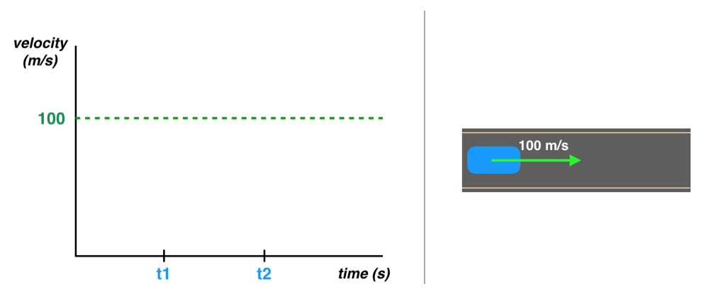
(Left) Graph of car velocity, (Right) a car going 100m/s on a road
Displacement
How much the car has moved is called the displacement and we already know how to calculate this!
We know, for example, that if the difference between t2 and t1 is one second, then we'll have moved 100m/sec*1sec = 100m. If the difference between t2 and t1 is two seconds, then we'll have moved 100m/sec*2sec = 200m.
The displacement is always = 100m/sec*(t2-t1).
Motion Model
Generally, for constant velocity, the motion model for displacement is:
displacement = velocity*dtWhere dt is calculus notation for "difference in time."
Area Under the Line
Going back to our graph, displacement can also be thought of as the area under the line and within the given time interval.
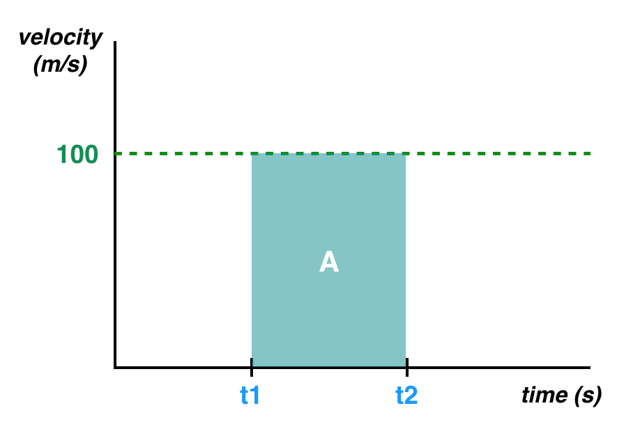
The area under the line, A, is equal to the displacement!
So, in addition to our motion model, we can also say that the displacement is equal to the area under the line!
displacement = AConstant Acceleration
The constant acceleration model is a little different; it assumes that our car is constantly accelerating; its velocity is changing at a constant rate.
Let's say our car has a velocity of 100m/s at time t1 and is accelerating at a rate of 10m/s^2.
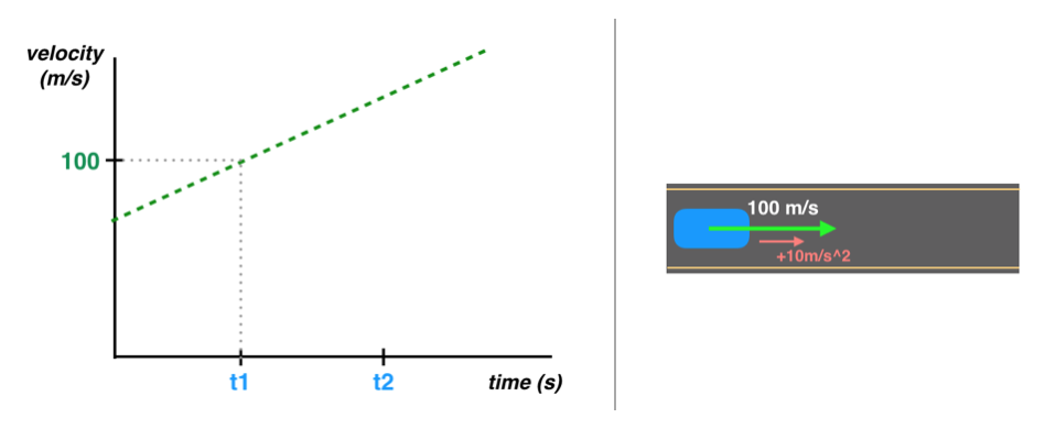
Changing Velocity
For this motion model, we know that the velocity is constantly changing, and increasing +10m/s each second. This can be represented by this kinematic equation (where dv is the change in velocity):
dv = acceleration*dtAt any given time, this can also be written as the current velocity is the initial velocity + the change in velocity over some time (dv):
v = initial_velocity + acceleration*dtDisplacement
Displacement can be calculated by finding the area under the line in between t1 and t2, similar to our constant velocity equation but a slightly different shape.
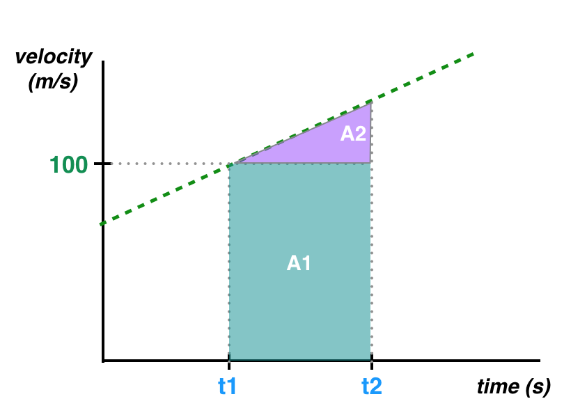
Area under the line, A1 and A2
This area can be calculated by breaking this area into two distinct shapes; a simple rectangle, A1, and a triangle, A2.
A1 is the same area as in the constant velocity model.
A1 = initial_velocity*dtIn other words, A1 = 100m/s*(t2-t1).
A2 is a little trickier to calculate, but remember that the area of a triangle is 0.5*width*height.
The width, we know, is our change in time (t2-t1) or dt.
And the height is the change in velocity over that time! From our earlier equation for velocity, we know that this value, dv, is equal to: acceleration*(t2-t1) or acceleration*dt
Now that we have the width and height of the triangle, we can calculate A2. Note that** is a Python operator for an exponent, so **2 is equivalent to ^2 in mathematics or squaring a value.
A2 = 0.5*acceleration*dt**2Motion Model
This means that our total displacement, A1+A2 ,can be represented by the equation:
displacement = initial_velocity*dt + 0.5*acceleration*dt**2We also know that our velocity over time changes according to the equation:
dv = acceleration*dtAnd these two equations, together, make up our motion model for constant acceleration.